We can use the cumulative frequency curves to find the median of a given grouped frequency distribution. The median refers to the middlemost value of the given data. This means that exactly half of the data lies above this value and exactly half of the data lies below it.
Steps to Find Median Using Ogive:
- We first calculate the less than cumulative frequencies (c.f.) in order to plot the less than cumulative frequency curve. This can be done by adding up the frequencies of the current and preceding class intervals.
- We construct the less than cumulative frequency curve. We plot ‘less than’ c.f. on the Y-axis against the upper limit of the corresponding class intervals on the X-axis and join the points so obtained by a smooth freehand curve.
- We now calculate the more than cumulative frequency. This can be done by adding the frequencies of the current and succeeding class intervals.
- We now plot the ‘more than’ ogive by joining the points obtained on plotting the ‘more than’ c.f. against the lower limit of the corresponding class by a smooth freehand curve.
- From the point of intersection of these two ogives, draw a line perpendicular to the X-axis. The abscissa (x-coordinate) of the point, where this perpendicular meets the X-axis, gives the value of the median.
We now explain how to carry out the above procedure by means of an example.
Example:
Consider the following grouped frequency distribution. We will calculate the median of the above distribution via the method indicated above.
| Class Interval | Frequency |
| Below 75 | 60 |
| 75 – 150 | 170 |
| 150 – 225 | 200 |
| 225 – 300 | 60 |
| 300 – 375 | 50 |
| 375 – 450 | 40 |
| More than 450 | 20 |
Step 1: We first calculate the less than cumulative frequencies as follows,
| Class Interval | Frequency | Less than c.f |
| Below 75 | 60 | 60 |
| 75 – 150 | 170 | 60+170 = 230 |
| 150 – 225 | 200 | 60 +170 + 200 = 430 |
| 225 – 300 | 60 | 60 +170 + 200 + 60 = 490 |
| 300 – 375 | 50 | 540 |
| 375 – 450 | 40 | 580 |
| More than 450 | 20 | 600 |
Step 2: We now calculate the more than cumulative frequencies by adding the current and succeeding frequencies.
| Class Interval | Frequency | More than c.f |
| Below 75 | 60 | 60 +170 + 200 + 60 + 50 + 40 +20 = 600 |
| 75 – 150 | 170 | 170 + 200 + 60 + 50 + 40 +20 = 540 |
| 150 – 225 | 200 | 200 + 60 + 50 + 40 +20 = 370 |
| 225 – 300 | 60 | 60 + 50 + 40 +20 = 170 |
| 300 – 375 | 50 | 50 + 40 +20 = 110 |
| 375 – 450 | 40 | 40 +20 = 60 |
| More than 450 | 20 | 20 |
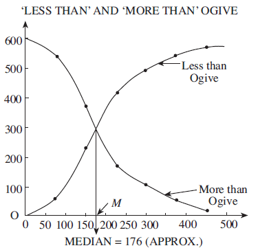
Step 3: We now draw the less than c.f curve and more than c.f. curve and drop a perpendicular from the point of intersection onto the X-axis. This gives us the required median. We conclude that the median of the given distribution is approximately 176.