We can calculate the residual value in regression analysis using the formula:
Residual = Actual value – Predicted Value.
We can find the predicted value of the dependent variable using the formula:
Y = β1X + β0.
Here, β1 and β0 are the regression coefficients for the linear model. We substitute the value of X in the above equation to find the predicted value for Y.
The Residual measures the distance between the actual value of the dependent variable compared to the predicted value obtained from the regression model. It is a measure of the error in the model.
Example 1:
Suppose that we are given the following set of data values about the marks obtained by 10 students in an exam vs the time spent studying for the exam.
| Time Spend Studying (in Hours) (X) | Marks Obtained (Y) |
| 4 | 38 |
| 5 | 42 |
| 6 | 56 |
| 7 | 59 |
| 8 | 61 |
| 11 | 68 |
| 13 | 72 |
| 14 | 78 |
| 18 | 86 |
| 21 | 95 |
Here, X = Time Spent Studying is the independent variable, and Y = Marks Obtained in the Exam is the dependent variable.
We can fit a regression model to the above data. For example, the linear model for the above set of data values is:
ŷ = 3.0716X + 32.63391.
Let us compute the residual value for the first pair of data values (X=4, Y=38).
We can find the predicted value ŷ (y hat) by substituting the value of X in the above regression equation. We compute that:
Predicted Value = 3.0716*4 + 32.63391 = 44.92031.
Also, the observed value of the dependent variable Y is:
Actual Observed Value Y = 38.
The residual can then be obtained by subtracting the actual value from the predicted value.
Residual = 38 – 44.92031 = -6.92031.
Notice that the residual value, in this case, is negative. This means that the model is giving us an overestimate for the actual value of Y.
Example 2:
Let us compute the residual value for the second pair of data values (X=5, Y=42).
We can find the predicted value by substituting the value X =5 in the regression equation. We compute that:
Predicted Value = 3.0716*5 + 32.63391 = 47.9919.
Also, the observed value of the dependent variable Y for the second data pair is Y = 42. The residual value is computed as:
Residual = Actual value – Predicted Value.
Residual = 42 – 47.9919 = -5.9919.
We can similarly find all residuals as follows:
Residual = Actual value – Predicted Value = Y – (β1X + β0).
Residual = Y – 3.0716X – 32.63391.
The residual values can be calculated as shown below:
| Time (X) | Marks (Y) | Residual = Y – 3.0716X – 32.63391 |
| 4 | 38 | 38 – 3.0716*4 – 32.63391 = -6.92031 |
| 5 | 42 | -5.9919 |
| 6 | 56 | 4.937 |
| 7 | 59 | 4.865 |
| 8 | 61 | 3.793 |
| 11 | 68 | 1.579 |
| 13 | 72 | -0.565 |
| 14 | 78 | 2.364 |
| 18 | 86 | -1.923 |
| 21 | 95 | -2.137 |
Understanding Residuals Graphically:
We can represent the residual graphically. The residuals represent the distance between of the actual data value from the “best fit line” of the data values.
The scatterplot and best fit line for the above set of data values looks like this:
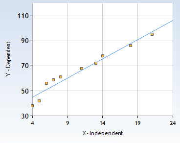
- The yellow dots in the above image represent the actual data values. Such a plot showing the relationship between the X and Y data values is known as a scatterplot.
- The best fit line passing through these points is drawn in such as way, that the distance between the line and the actual value is minimized.
- The residual value is equal to the vertical distance between the yellow dots and the blue line.
- In regression analysis, our aim is to find the equation of a line that is the best fit for the data value. This is done by minimizing the square of the residual values. This method of obtaining the regression equations is known as the least squares method.
