The binomial and normal distributions are probability distributions that have a wide range of applications in statistics and real life. The main differences between the binomial and normal distributions are the following.
1) Discrete vs Continuous:
The main difference between the binomial and normal distributions is that the binomial distribution is a discrete distribution whereas the normal distribution is a continuous distribution.
This means that a binomial random variable can only take integer values such as 1, 2, 3, etc. whereas the normal variable can take any real number value such as 1.2 or 2.314, etc.
For example, the height of the human population is normally distributed. As we know the height of a person can take any decimal value such as 1.72cm, 1.82cm, etc.
2) Range of the Distribution:
The second difference between them is that a binomial random variable has a finite range whereas the normal distribution has an infinite range.
A binomial random variable can only take finitely many values 0, 1, 2,…., n. For example, suppose that a coin is tossed 10 times. The number of heads obtained is a random variable following the binomial distribution. It is clear that the possible values for the number of heads obtained are 0, 1,2,…,10.
On the other hand, a normal random variable can take any value between minus infinity to plus infinity, and therefore its range is unbounded.
In fact, the range of the normal distribution is uncountably infinite.
3) When to use Normal vs Binomial distribution?
The binomial distribution is limited in its applications. It is only used in situations where a trial can have only two possible outcomes – success or failure.
For example, when tossing a coin many times we use the binomial distribution to calculate probabilities (since tossing a coin has only two outcomes – heads or tails). It can be used to calculate the probability of ‘r’ successes out of ‘n’ trials.
On the other hand, the normal distribution finds many applications in real-life situations such as modeling the height or weight distribution of a population.
One of the most important applications of the normal distribution is the central limit theorem. The central limit theorem allows us to make conclusions about an unknown population mean on the basis of a randomly selected sample. The central limit theorem says that the sample mean follows the normal distribution.
The normal distribution can also be used to calculate probabilities for binomial distribution using the method of normal approximation to the binomial.
Normal PDF vs Binomial PDF:
The PDF (probability distribution function) for a binomial random variable with parameters ‘n’ and ‘p’ is given by the formula,
f(x) = nCx px (1-p)n-x where, x = 0, 1, 2,…n.
- Here, n is the total number of trials.
- p is the probability of success.
- x is the number of successes.
The PDF (probability density function) for a normal random variable with mean μ and variance σ2 is given by the formula,
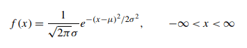
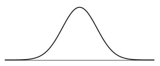
The PDF of the normal distribution is in the shape of a bell-shaped curve.
Binomial vs Normal Variance:
The mean and variance of the binomial distribution are obtained by multiplying the parameters of the distribution as shown below:
Mean = E(X) = np.
Variance = V(X) = np(1-p).
On the other hand, the mean and variance of the normal distribution are simply equal to the parameters of the normal distribution.
Mean = E(X) = μ.
Variance = V(X) = σ2.