This non-parametric test for two samples was described by Wilcoxon and studied by Mann and Whitney. It is the most widely used test as an alternative to the t-test when we do not make the t-test assumptions about the parent population.
This test is used to test whether two independent samples come from the same population in situations where you don’t have interval or ratio data (and thus can’t use the t-test).
This test can be directly applied if the data is ordinal. If the data is not ordinal we can rank the data. We then work with these ranks rather than the original data points.
The value of the test statistic can be calculated using the formula,
U= NANB + NA(NA+1)/2 – RA.
where RA is the sum of the ranks in column A, NA is the number of scores in column A, and NB is the number of scores in column B.
We now explain how to carry out the test in Excel with the help of an example.
How to Perform the Mann-Whitney Test in Excel:
Suppose that a group of 40 people is divided into two equal groups. One group watches a stressful movie while the other watches a stressful cartoon. They then rate the degree of their stress after watching on a scale of 1 to 100.
Our null hypothesis, in this case, is that we expect people to experience the same degree of stress on watching either the movie or the cartoon. The alternative hypothesis is that the stress would be higher after the stressful movie. We carry out the test as follows.
Step 1: We first enter the data values. We can see that the data values are entered in columns A and B in the below image.
Step 2: We assign ranks to the data values. The ranks can be obtained using the RANK.AVG command.
In cell D2, type the command =RANK.AVG(A2,$A$2:$B$21,1) and then autofill columns D and E. The ranks are obtained in columns D and E as shown in the image below.
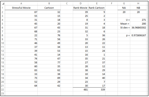
Step 3: Input the values of NA and NB in the cells G2 and H2 as shown in the image. Then calculate the value of the test statistic using the following formula in cell H4,
=NA*NB +((NA*(NA+1))/2)-E22
Step 4: Calculate the mean and standard deviation for U. The mean is calculated in cell H5 using the formula,
=(NA*NB)/2
The standard deviation is calculated in cell H6 using the formula,
=SQRT((NA*NB*(NA+NB+1))/12)
Step 5: We calculate the p-values with help of the above values. We use the following command.
=NORM.DIST(H4,H5,H6,TRUE)
The result of 0.97 is obtained in cell H8. This means that the p-value is equal to 1- 0.97 =0.03. Since the p-value is less than 0.05 we reject the null hypothesis.
This means that the movie and cartoon do not produce equal amounts of stress. We conclude that the movie produces much more stress compared to the cartoon.