What is the Geometric Distribution? (with Examples)

The geometric distribution is a discrete probability distribution that is used to calculate the probability of failing in a certain number of successive Bernoulli trials before success is achieved.

How is the geometric distribution obtained?

Suppose an archer is trying to hit a target. Either he hits the target or fails to do so. If he fails he tries again. Let us assume that the probability of hitting the target in each trial attempt is fixed, say p.

We further assume that each trial is independent. We wish to calculate the probability that the man fails ‘x-1’ number of times before he succeeds in hitting the target.

Since the probability of failure is (1-p) and failure occurs ‘x-1’ number of times followed by a success whose probability is p we use the multiplication law to obtain the required probability.

Note that we can use the law of multiplication since we are assuming that the successive trials are independent.

Hence, the required probability = p*(1-p)^X-1  which is precisely the probability mass function of the geometric distribution.

Probability Mass Function(PMF) of the Geometric Distribution:

The probability mass function of the geometric distribution is given by the formula:

P(X=x) =  p*(1-p)^X-1 if x=0,1,2,3,…

We sometimes use the notation q=1-p.

Note that as expected the total probability adds up to 1 by the well-known formula for the summation of an infinite geometric series.

In fact, this is the reason why the distribution is called the geometric distribution.                                                                   

Expected Value and Variance of Geometric Distribution: (with Proof):

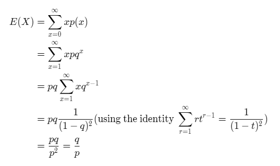
The mean/expected value of the geometric distribution is given by the formula:

E(X)= (1-p)/p.

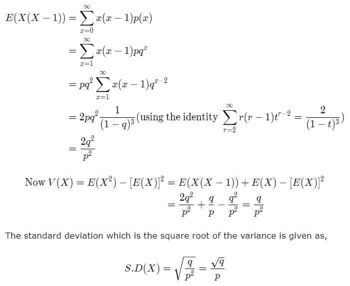
The variance of the geometric distribution is given by the formula:

V(X)= (1-p)/p².

The derivation of the mean and the expected value is shown below.

Example:

Suppose an archer is trying to hit a target. The probability that he hits the target in a particular trial is 30%. Calculate the probability that he succeeds on the fifth attempt. Also, calculate the mean and the variance.

Solution: Given X=5 and p=0.30. We substitute the data in the above probability mass function to get,

P(X=5)=(0.30)(0.70)⁵=0.050421.

We calculate the mean and variance using the following formulae,

Mean = (1-p)/p = 1-0.3/0.3 = 2.3334.

Variance = (1-p)/p² = 0.7/0.09 = 7.78.

Lack of Memory Property of the Geometric Distribution:

The geometric distribution has the memoryless property.

Suppose an event E can occur at one of the times t = 0, 1, 2, … and the occurrence (waiting) time X follows the geometric distribution.

Suppose we know that the event E has not occurred before k, i.e., X ≥ k.

Let Y – X – k. Thus Y is the amount of additional time needed for E to occur. We can show that,

P(Y=t|X ≥ k) = P(X=t),

which implies that the additional time to wait has the same distribution as the initial time to wait.

Since the distribution does not depend upon k, it “lacks memory” of how much we shifted the time origin.

If a person ‘B’ were waiting for event E and is replaced by person ‘C’ immediately before time k, then the waiting time distribution of ‘C’ is the same as that of ‘B’.

Geometric vs Binomial Distribution:

1. If a random variable follows geometric distribution it can take any integer value from 0 to infinity. On the other hand, the range of a binomial random variable is a finite set of values 0, 1, …., n.
2. The geometric distribution has the memoryless property whereas the binomial distribution does not have the memoryless property.
3. The sum of “k” independent and identically distributed geometric random variables follows a negative binomial distribution. The sum of “k” i.i.d random variables once again follows a binomial distribution.