A left skewed histogram is a histogram that attains a peak (which is the mode) towards the right side of the graph and has a “tail” towards the left side.
This means that the data has contains a greater number of larger values compared to smaller values.
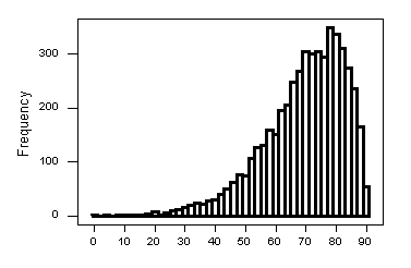
The above image is an example of a left skewed histogram. We can see that it has a “peak” towards the right with its mode lying somewhere between 70 and 80.
The graph has its “tail” towards the left side. We use the side in which the tail lies to decide whether the histogram is left skewed or right skewed.
If a histogram is skewed towards the left, we say that the histogram has negative skewness and that the distribution is negatively skewed.
Relationship between Mean, Median, and Mode in a Left Skewed Histogram:
We have the following relationship between the mean, median, and mode.
Mean≤Median≤Mode.
The reason for the mean being smaller than the median and the mode is that in a left skewed distribution, there is a greater frequency of larger values which increases the median and mode of the data.
The value of skewness will always be negative for a left skewed histogram because the mean is less than the mode in a left skewed distribution.
Real-Life Example of left-skewed data:
The death rates of individuals compared with age is an example of left skewed data. If we were to plot the age on the X- axis and the number of deaths in that age group on the Y-axis we would get a left skewed histogram.
This is because there will be greater number of deaths among the older population. There will be relatively less frequency of deaths among the younger population.
Construction of a left skewed histogram:
Consider the following data showing the marks obtained by a group of students in an exam worth 100 points.
| Class Intervals (Marks obtained) | Frequency (Number of students) |
| 0-10 | 1 |
| 10-20 | 1 |
| 20-30 | 2 |
| 30-40 | 4 |
| 40-50 | 7 |
| 50-60 | 14 |
| 60-70 | 16 |
| 70-80 | 22 |
| 80-90 | 21 |
| 90-100 | 15 |
We plot the above data and obtain the following histogram,
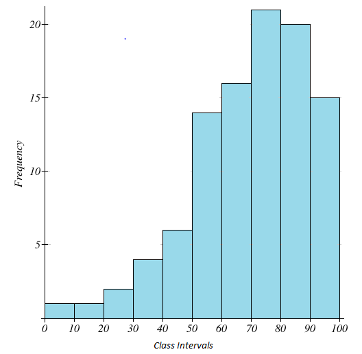
Once again, notice that the mode of the histogram lies towards the right and the tail lies towards the left.